Fitting Types

Fit (LeastSquares)

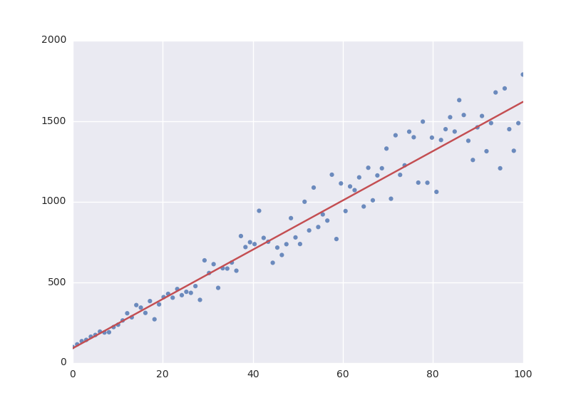
The default fitting object does least-squares fitting:

from symfit.api import Parameter, Variable, Fit
import numpy as np

# Define a model to fit to.
a = Parameter()
b = Parameter()
x = Variable()
model = a * x + b

# Generate some data
xdata = np.linspace(0, 100, 100) # From 0 to 100 in 100 steps
a_vec = np.random.normal(15.0, scale=2.0, size=(100,))
b_vec = np.random.normal(100.0, scale=2.0, size=(100,))
ydata = a_vec * xdata + b_vec # Point scattered around the line 5 * x + 105

fit = Fit(model, xdata, ydata)
fit_result = fit.execute()

Fit currently simply wraps LeastSquares. This might be changed in the future to it determining which fit would work best for the current data and then just trying the best option.

Likelihood

Given a dataset and a model, what values should the model’s parameters have to make the observed data most likely? This is the principle of maximum likelihood and the question the Likelihood object can answer for you.

Example:

from symfit.api import Parameter, Variable, Likelihood, exp
import numpy as np

# Define the model for an exponential distribution (numpy style)
beta = Parameter()
x = Variable()
model = (1 / beta) * exp(-x / beta)

# Draw 100 samples from an exponential distribution with beta=5.5
data = np.random.exponential(5.5, 100)

# Do the fitting!
fit = Likelihood(model, data)
fit_result = fit.execute()

Off-course fit_result is a normal FitResults object. Because scipy.optimize.minimize is used to do the actual work, bounds on parameters, and even constraints are supported. For more information on this subject, check out symfit‘s Minimize.

Minimize/Maximize

Minimize or Maximize a model subject to bounds and/or constraints. It is a wrapper to scipy.optimize.minimize. As an example I present an example from the scipy docs.

Suppose we want to maximize the following function:

\[f(x,y) = 2xy + 2x - x^2 - 2y^2\]

Subject to the following constraits:

\[x^3 - y = 0\]

\[\begin{split}y - 1 >= 0\end{split}\]

In SciPy code the following lines are needed:

def func(x, sign=1.0):
    """ Objective function """
    return sign*(2*x[0]*x[1] + 2*x[0] - x[0]**2 - 2*x[1]**2)

def func_deriv(x, sign=1.0):
    """ Derivative of objective function """
    dfdx0 = sign*(-2*x[0] + 2*x[1] + 2)
    dfdx1 = sign*(2*x[0] - 4*x[1])
    return np.array([ dfdx0, dfdx1 ])

cons = ({'type': 'eq',
         'fun' : lambda x: np.array([x[0]**3 - x[1]]),
         'jac' : lambda x: np.array([3.0*(x[0]**2.0), -1.0])},
        {'type': 'ineq',
         'fun' : lambda x: np.array([x[1] - 1]),
         'jac' : lambda x: np.array([0.0, 1.0])})

res = minimize(func, [-1.0,1.0], args=(-1.0,), jac=func_deriv,
               constraints=cons, method='SLSQP', options={'disp': True})

Takes a couple of readthroughs to make sense, doesn’t it? Let’s do the same problem in symfit:

x = Parameter()
y = Parameter()
model = 2*x*y + 2*x - x**2 -2*y**2
constraints = [
  x**3 - y == 0,
  y - 1 >= 0,
]

fit = Maximize(model, constraints=constraints)
fit_result = fit.execute()

Done! symfit will determine all derivatives automatically, no need for you to think about it.

Warning

You might have noticed that x and y are Parameter‘s in the above problem, which may stike you as weird. However, it makes perfect sence because in this problem they are parameters to be optimised, not variables. Furthermore, this way of defining it is consistent with the treatment of Variable‘s and Parameter‘s in symfit. Be aware of this when using these objects, as the whole process won’t work otherwise.