Fitting Types
Fit (LeastSquares)
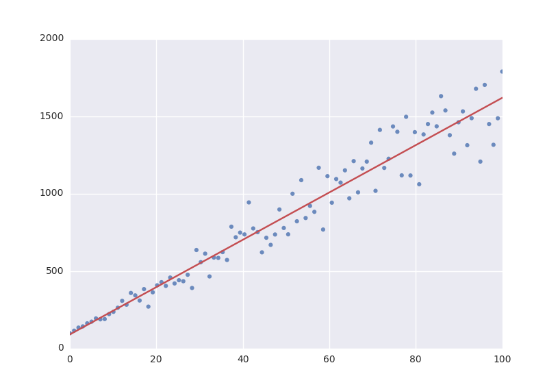
The default fitting object does least-squares fitting:
from symfit import parameters, variables, Fit
import numpy as np

# Define a model to fit to.
a, b = parameters('a, b')
x = variables('x')
model = a * x + b

# Generate some data
xdata = np.linspace(0, 100, 100) # From 0 to 100 in 100 steps
a_vec = np.random.normal(15.0, scale=2.0, size=(100,))
b_vec = np.random.normal(100.0, scale=2.0, size=(100,))
ydata = a_vec * xdata + b_vec # Point scattered around the line 5 * x + 105

fit = Fit(model, xdata, ydata)
fit_result = fit.execute()
The Fit object also supports standard deviations. In order to provide these, it’s nicer to use a named model:
a, b = parameters('a, b')
x, y = variables('x, y')
model = {y: a * x + b}

fit = Fit(model, x=xdata, y=ydata, sigma_y=sigma)
Symfit assumes these sigma to be from measurement errors by default, and not just as a relative weight.
This means the standard deviations on parameters are calculated assuming the absolute size
of sigma is significant. This is the case for measurement errors and therefore for most use cases symfit was
designed for. If you only want to use the sigma for relative weights, then you can use absolute_sigma=False as a
keyword argument.
Please note that this is the opposite of the convention used by scipy’s curve_fit.
Looking through their mailing list this seems to have been implemented the ‘wrong’ way
for historical reasons, and was understandably never changed so as not to loose backwards compatibility.
Since this is a new project, we don’t have that problem.
Fit currently simply wraps NumericalLeastSquares, but might become more intelligent in the future.
Likelihood
Given a dataset and a model, what values should the model’s parameters have to make the observed data most likely? This is the principle of maximum likelihood and the question the Likelihood object can answer for you.
Example:
from symfit import Parameter, Variable, Likelihood, exp
import numpy as np

# Define the model for an exponential distribution (numpy style)
beta = Parameter()
x = Variable()
model = (1 / beta) * exp(-x / beta)

# Draw 100 samples from an exponential distribution with beta=5.5
data = np.random.exponential(5.5, 100)

# Do the fitting!
fit = Likelihood(model, data)
fit_result = fit.execute()
Off-course fit_result is a normal FitResults object. Because scipy.optimize.minimize is used to do the actual work, bounds on parameters, and even constraints are supported. For more information on this subject, check out symfit‘s Minimize.
Minimize/Maximize
Minimize or Maximize a model subject to bounds and/or constraints. It is a wrapper to scipy.optimize.minimize. As an
example I present an example from the scipy docs.
Suppose we want to maximize the following function:
Subject to the following constraints:
In SciPy code the following lines are needed:
def func(x, sign=1.0):
    """ Objective function """
    return sign*(2*x[0]*x[1] + 2*x[0] - x[0]**2 - 2*x[1]**2)

def func_deriv(x, sign=1.0):
    """ Derivative of objective function """
    dfdx0 = sign*(-2*x[0] + 2*x[1] + 2)
    dfdx1 = sign*(2*x[0] - 4*x[1])
    return np.array([ dfdx0, dfdx1 ])

cons = ({'type': 'eq',
        'fun' : lambda x: np.array([x[0]**3 - x[1]]),
        'jac' : lambda x: np.array([3.0*(x[0]**2.0), -1.0])},
        {'type': 'ineq',
        'fun' : lambda x: np.array([x[1] - 1]),
        'jac' : lambda x: np.array([0.0, 1.0])})

res = minimize(func, [-1.0,1.0], args=(-1.0,), jac=func_deriv,
               constraints=cons, method='SLSQP', options={'disp': True})
Takes a couple of read-throughs to make sense, doesn’t it? Let’s do the same problem in symfit:
from symfit import parameters, Maximize, Eq, Ge

x, y = parameters('x, y')
model = 2*x*y + 2*x - x**2 -2*y**2
constraints = [
    Eq(x**3 - y, 0),
    Ge(y - 1, 0),
]

fit = Maximize(model, constraints=constraints)
fit_result = fit.execute()
Done! symfit will determine all derivatives automatically, no need for you to think about it.
Warning
You might have noticed that x and y are Parameter‘s in the above problem, which may strike you as weird.
However, it makes perfect sense because in this problem they are parameters to be optimised, not variables.
Furthermore, this way of defining it is consistent with the treatment of Variable‘s and Parameter‘s in symfit.
Be aware of this when using Minimize, as the whole process won’t work otherwise.
How Does Fit Work?
How does Fit get from a (named) model and some data to a fit? Consider the following example:
from symfit.api import parameters, variables, Fit

a, b = parameters('a, b')
x, y = variables('x, y')
model = {y: a * x + b}

fit = Fit(model, x=x_data, y=y_data, sigma_y=sigma_data)
fit_result = fit.execute()
The first thing symfit does is build \(\chi^2\) for your model:
chi_squared = sum((y - f)**2/sigmas[y]**2 for y, f in model.items())
In this line sigmas is a dict which contains all vars that where given a value, or returns 1 otherwise.
This \(\chi^2\) is then transformed into a python function which can then be used to do the numerical calculations:
vars, params = seperate_symbols(chi_squared)
py_chi_squared = lambdify(vars + params, chi_squared)
We are now almost there. Just two steps left. The first is to wrap all the data into the py_chi_squared function using partial into the function to be optimized:
from functools import partial

error = partial(py_chi_squared, **data_per_var)
where data_per_var is a dict containing variable names: value pairs.
Now all that is left is to call leastsqbound and have it find the best fit parameters:
best_fit_parameters, covariance_matrix = leastsqbound(
  error,
  self.guesses,
  self.eval_jacobian,
  self.bounds,
)
That’s it! Finally there are some steps to generate a FitResult object, but these are not important for our current discussion.
What if the model is unnamed?
Then you’ll have to use the ordering. Variables throughout symfit‘s objects are internally ordered in the following
way: first independent variables, then dependent variables, then sigma variables, and lastly parameters when applicable.
Within each group alphabetical ordering applies.
It is therefore always possible to assign data to variables in an unambiguis way using this ordering. In the above example:
fit = Fit(model, x_data, y_data, sigma_data)