Tutorial
Simple Example
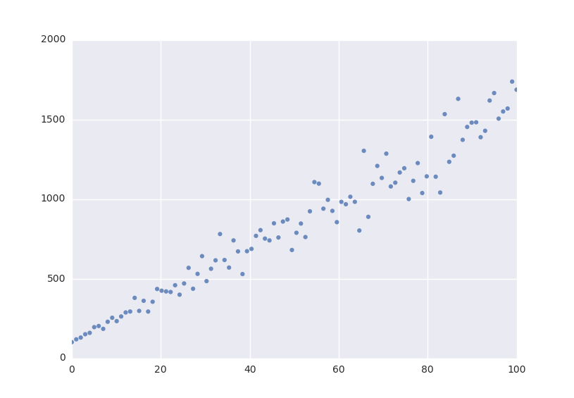
The example below shows how easy it is to define a model that we could fit to.
from symfit.api import Parameter, Variable

a = Parameter()
b = Parameter()
x = Variable()
model = a * x + b
Lets fit this model to some generated data.
from symfit.api import Fit
import numpy as np

xdata = np.linspace(0, 100, 100) # From 0 to 100 in 100 steps
a_vec = np.random.normal(15.0, scale=2.0, size=(100,))
b_vec = np.random.normal(100.0, scale=2.0, size=(100,))
ydata = a_vec * xdata + b_vec # Point scattered around the line 5 * x + 105

fit = Fit(model, xdata, ydata)
fit_result = fit.execute()
Printing fit_result will give a full report on the values for every parameter, including the uncertainty, and quality of the fit.
Initial Guess
For fitting to work as desired you should always give a good initial guess for a parameter.
The Parameter object can therefore be initiated with the following keywords:
valuethe initial guess value.minMinimal value for the parameter.maxMaximal value for the parameter.fixedFix the value of the parameter during the fitting tovalue.
In the example above, we might change our Parameter‘s to the following after looking at a plot of the data:
k = Parameter(value=4, min=3, max=6)

l, m = parameters('b, c')
l.value = 60
l.fixed = True
Accessing the Results
A call to Fit.execute() returns a FitResults instance.
This object holds all information about the fit.
The fitting process does not modify the Parameter objects.
In the above example, k.value will still be 4.0 and not the value we obtain after fitting. To get the value of fit parameters we can do:
>>> print(fit_result.params.a)
>>> 14.66946...
>>> print(fit_result.params.a_stdev)
>>> 0.3367571...
>>> print(fit_result.params.b)
>>> 104.6558...
>>> print(fit_result.params.b_stdev)
>>> 19.49172...
>>> print(fit_result.r_squared)
>>> 0.950890866472
For more FitResults, see the API docs.
Evaluating the Model
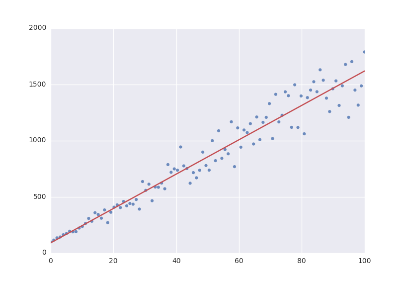
With these parameters, we could now evaluate the model with these parameters so we can make a plot of it. In order to do this, we simply call the model with these values:
import matplotlib.pyplot as plt

y = model(x=xdata, a=fit_result.params.a, b=fit_result.params.b)
plt.plot(xdata, y)
plt.show()
The model has to be called by keyword arguments to prevent any ambiguity. So the following does not work:
y = model(xdata, fit_result.params.a, fit_result.params.b)
To make life easier, there is a nice shorthand notation to immediately use a fit result:
y = model(x=xdata, **fit_result.params)
This unpacks the .params object as a dict. For more info view ParameterDict.
Named Models
More complicated models are also relatively easy to deal with by using named models. Let’s try our luck with a bivariate normal distribution:
from symfit import parameters, variables, exp, pi, sqrt

x, y, p = variables('x, y, p')
mu_x, mu_y, sig_x, sig_y, rho = parameters('mu_x, mu_y, sig_x, sig_y, rho')

z = (x - mu_x)**2/sig_x**2 + (y - mu_y)**2/sig_y**2 - 2 * rho * (x - mu_x) * (y - mu_y)/(sig_x * sig_y)
model = {p: exp(- z / (2 * (1 - rho**2))) / (2 * pi * sig_x * sig_y * sqrt(1 - rho**2))}

fit = Fit(model, x=xdata, y=ydata, p=pdata)
By using the magic of named models, the flow of information is still very clear, even with such a complicated function.
This syntax also supports vector valued functions:
model = {y_1: a * x**2, y_2: 2 * x * b}
One thing to note about such models is that now model(x=xdata) obviously no longer works as type(model) == dict.
There is a prevered way to resolve this. If any kind of fitting object has been initiated, it will have a .model atribute
containing an instance of Model. This can again be called:
model = {y_1: a * x**2, y_2: 2 * x * b}
fit = Fit(model, x=xdata)
fit_result = fit.execute()

y_1, y_2 = fit.model(x=xdata, **fit_result.params)
This returns a tuple with the components evaluated so through the magic of tuple unpacking``y_1`` and y_2 contain the
evaluated fit. Nice!
If for some reason no Fit is initiated you can make a Model object yourself:
from symfit import Model

model_dict = {y_1: a * x**2, y_2: 2 * x * b}
model = Model.from_dict(model_dict)

y_1, y_2 = fit.model(x=xdata, a=2.4, b=0.1)
symfit exposes sympy.api
symfit exposes the sympy api as well, so mathematical expressions such as exp, sin and pi are importable
from symfit as well. For more, read the sympy docs.