Example: Interactive Guesses in N dimensions

Below is an example in which the initial guesses module is used to help fit a function that depends on more than one independent variable:

# SPDX-FileCopyrightText: 2014-2020 Martin Roelfs
#
# SPDX-License-Identifier: MIT

# -*- coding: utf-8 -*-

from symfit import variables, Parameter, exp, Fit, Model
from symfit.distributions import Gaussian
from symfit.contrib.interactive_guess import InteractiveGuess
import numpy as np


x, y, z = variables('x, y, z')
mu_x = Parameter('mu_x', 10)
mu_y = Parameter('mu_y', 10)
sig_x = Parameter('sig_x', 1)
sig_y = Parameter('sig_y', 1)



model = Model({z: Gaussian(x, mu_x, sig_x) * Gaussian(y, mu_y, sig_y)})
x_data = np.linspace(0, 25, 50)
y_data = np.linspace(0, 25, 50)
x_data, y_data = np.meshgrid(x_data, y_data)
x_data = x_data.flatten()
y_data = y_data.flatten()
z_data = model(x=x_data, y=y_data, mu_x=5, sig_x=0.3, mu_y=10, sig_y=1).z

guess = InteractiveGuess(model, x=x_data, y=y_data, z=z_data)
guess.execute()
print(guess)

fit = Fit(model, x=x_data, y=y_data, z=z_data)
fit_result = fit.execute()
print(fit_result)

This is a screenshot of the interactive guess window:

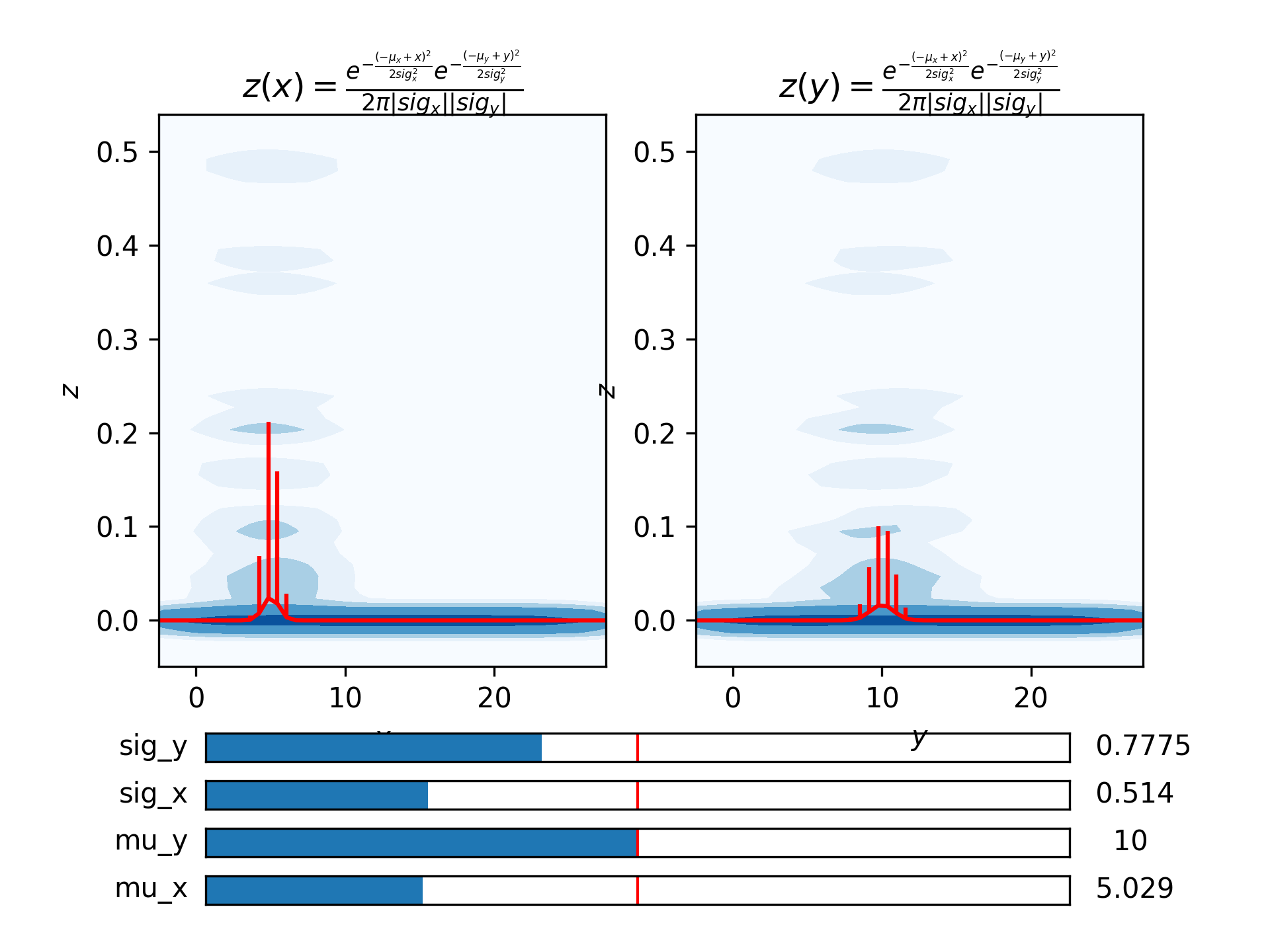
In the window you can see the range the provided data spans as a contourplot on the background. The evaluated models is shown as red lines. By default your proposed model is evaluated at \(50^n\) points for \(n\) independent variables, with 50 points per dimension. So in the example this is at 50 values of x and 50 values of y. The error bars on the points plotted are taken from the spread in z that comes from the spread in data in the other dimensions (y and x respectively). The error bars correspond (by default) to the 90% percentile.

By using the sliders, you can interactively play with the initial guesses until it is close enough. Then after closing the window, this initial values are set for the parameters, and the fit can be performed.