Example: Interactive Guesses ODE

Below is an example in which the initial guesses module is used to help solve an ODE problem.

# SPDX-FileCopyrightText: 2014-2020 Martin Roelfs
#
# SPDX-License-Identifier: MIT

#!/usr/bin/env python3
# -*- coding: utf-8 -*-
from symfit import variables, Parameter, Fit, D, ODEModel
import numpy as np
from symfit.contrib.interactive_guess import InteractiveGuess


# First order reaction kinetics. Data taken from
# http://chem.libretexts.org/Core/Physical_Chemistry/Kinetics/Rate_Laws/The_Rate_Law
tdata = np.array([0, 0.9184, 9.0875, 11.2485, 17.5255, 23.9993, 27.7949,
                  31.9783, 35.2118, 42.973, 46.6555, 50.3922, 55.4747, 61.827,
                  65.6603, 70.0939])
concentration = np.array([0.906, 0.8739, 0.5622, 0.5156, 0.3718, 0.2702, 0.2238,
                          0.1761, 0.1495, 0.1029, 0.086, 0.0697, 0.0546, 0.0393,
                          0.0324, 0.026])

# Define our ODE model
A, t = variables('A, t')
k = Parameter('k')
model = ODEModel({D(A, t): - k * A}, initial={t: tdata[0], A: concentration[0]})

guess = InteractiveGuess(model, A=concentration, t=tdata, n_points=250)
guess.execute()
print(guess)

fit = Fit(model, A=concentration, t=tdata)
fit_result = fit.execute()
print(fit_result)

This is a screenshot of the interactive guess window:

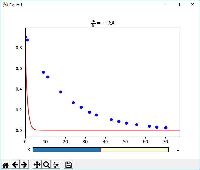
By using the sliders, you can interactively play with the initial guesses until it is close enough. Then after closing the window, this initial value is set for the parameter, and the fit can be performed.