Global minimization: Skewed Mexican hat

In this example we will demonstrate the ease of performing global minimization using symfit. In order to do this we will have a look at a simple skewed mexican hat potential, which has a local minimum and a global minimum. We will then use DifferentialEvolution to find the global minimum.

from symfit import Parameter, Variable, Model, Fit, solve, diff, N, re
from symfit.core.minimizers import DifferentialEvolution, BFGS
import numpy as np
import matplotlib.pyplot as plt

First we define a model for the skewed mexican hat.

x = Parameter('x')
x.min, x.max = -100, 100
y = Variable('y')
model = Model({y: x**4 - 10 * x**2 + 5 * x})  # Skewed Mexican hat
print(model)

[y(; x) = x**4 - 10*x**2 + 5*x]

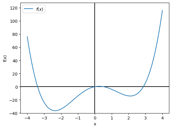
Let us visualize what this potential looks like.

xdata = np.linspace(-4, 4, 201)
ydata = model(x=xdata).y

plt.axhline(0, color='black')
plt.axvline(0, color='black')
plt.plot(xdata, ydata, label=r'$f(x)$')
plt.xlabel('x')
plt.ylabel('f(x)')
plt.ylim(1.1 * ydata.min(), 1.1 * ydata.max())
plt.legend()

<matplotlib.legend.Legend at 0x7fbd20702e10>

Using sympy, it is easy to solve the solution analytically, by finding the places where the gradient is zero.

sol = solve(diff(model[y], x), x)
# Give numerical value
sol = [re(N(s)) for s in sol]
sol

[0.253248404857807, 2.09866205647752, -2.35191046133532]

Without providing any initial guesses, symfit finds the local minimum. This is because the initial guess is set to 1 by default.

fit = Fit(model)
fit_result = fit.execute()
print('exact value', sol[1])
print('num  value ', fit_result.value(x))

exact value 2.09866205647752
num  value  2.09866205722533

Let’s use DifferentialEvolution instead.

fit = Fit(model, minimizer=DifferentialEvolution)
fit_result = fit.execute()
print('exact value', sol[2])
print('num  value ', fit_result.value(x))

exact value -2.35191046133532
num  value  -2.3529107622872747

Using DifferentialEvolution, we find the correct global minimum. However, it is not exactly the same as the analytical solution. This is because DifferentialEvolution is expensive to perform, and therefore does not solve to high precision by default. We could demand a higher precission from DifferentialEvolution, but this isn’t worth the high computational cost. Instead, we will just tell symfit to perform DifferentialEvolution, followed by BFGS.

fit = Fit(model, minimizer=[DifferentialEvolution, BFGS])
fit_result = fit.execute()
print('exact value', sol[2])
print('num  value ', fit_result.value(x))

exact value -2.35191046133532
num  value  -2.351910461335213

We see that now the proper solution has been found to much higher precision.