Example: Piecewise model using CallableNumericalModel
Below is an example of how to use the
symfit.core.models.CallableNumericalModel. This class allows you to
provide custom callables as your model, while still allowing clean interfacing
with the symfit API.
These models also accept a mixture of symbolic and callable components, as will
be demonstrated below. This allows the power-user great flexibility, since it is
still easy to interface with symfit’s constraints, minimizers, etc.
from symfit import variables, parameters, Fit, D, ODEModel, CallableNumericalModel
import numpy as np
import matplotlib.pyplot as plt

def nonanalytical_func(x, a, b):
    """
    This can be any pythonic function which should be fitted, typically one
    which is not easily written or supported as an analytical expression.
    """
    # Do your non-trivial magic here. In this case a Piecewise, although this
    # could also be done symbolically.
    y = np.zeros_like(x)
    y[x > b] = (a * (x - b) + b)[x > b]
    y[x <= b] = b
    return y

x, y1, y2 = variables('x, y1, y2')
a, b = parameters('a, b')

mixed_model = CallableNumericalModel(
    {y1: nonanalytical_func, y2: x ** a},
    connectivity_mapping={y1: {x, a, b}}
)

# Generate data
xdata = np.linspace(0, 10)
y1data, y2data = mixed_model(x=xdata, a=1.3, b=4)
y1data = np.random.normal(y1data, 0.1 * y1data)
y2data = np.random.normal(y2data, 0.1 * y2data)

# Perform the fit
b.value = 3.5
fit = Fit(mixed_model, x=xdata, y1=y1data, y2=y2data)
fit_result = fit.execute()
print(fit_result)

# Plotting, irrelevant to the symfit part.
y1_fit, y2_fit, = mixed_model(x=xdata, **fit_result.params)
plt.scatter(xdata, y1data)
plt.plot(xdata, y1_fit, label=r'$y_1$')
plt.scatter(xdata, y2data)
plt.plot(xdata, y2_fit, label=r'$y_2$')
plt.legend(loc=0)
plt.show()
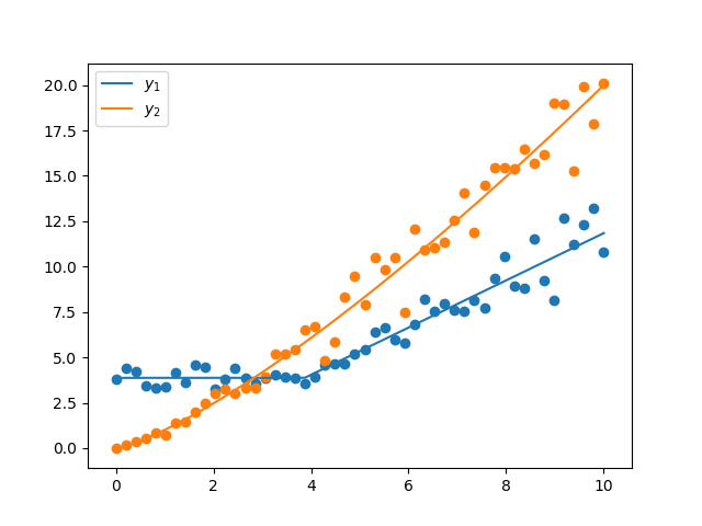
This is the resulting fit: