Example: Polynomial Surface Fit
In this example, we want to fit a polynomial to a 2D surface. Suppose the surface is described by
\[f(x) = x^2 + y^2 + 2 x y\]
A fit to such data can be performed as follows:
from symfit import Poly, variables, parameters, Model, Fit
import numpy as np
import matplotlib.pyplot as plt
import seaborn as sns
x, y, z = variables('x, y, z')
c1, c2 = parameters('c1, c2')
# Make a polynomial. Note the `as_expr` to make it symfit friendly.
model_dict = {
z: Poly( {(2, 0): c1, (0, 2): c1, (1, 1): c2}, x ,y).as_expr()
}
model = Model(model_dict)
print(model)
# Generate example data
x_vec = np.linspace(-5, 5)
y_vec = np.linspace(-10, 10)
xdata, ydata = np.meshgrid(x_vec, y_vec)
zdata = model(x=xdata, y=ydata, c1=1.0, c2=2.0).z
zdata = np.random.normal(zdata, 0.05 * zdata) # add 5% noise
# Perform the fit
fit = Fit(model, x=xdata, y=ydata, z=zdata)
fit_result = fit.execute()
zfit = model(x=xdata, y=ydata, **fit_result.params).z
print(fit_result)
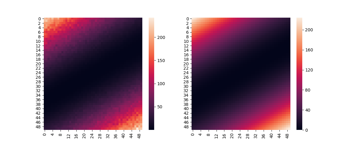
fig, (ax1, ax2) = plt.subplots(1, 2)
sns.heatmap(zdata, ax=ax1)
sns.heatmap(zfit, ax=ax2)
plt.show()
This code prints:
z(x, y; c1, c2) = c1*x**2 + c1*y**2 + c2*x*y

Parameter Value        Standard Deviation
c1        9.973489e-01 1.203071e-03
c2        1.996901e+00 3.736484e-03
Fitting status message: Optimization terminated successfully.
Number of iterations:   6
Regression Coefficient: 0.9952824293713467