Example: Matrix Equations using Tikhonov Regularization

This is an example of the use of matrix expressions in symfit models. This is illustrated by performing an inverse Laplace transform using Tikhonov regularization, but this could be adapted to other problems involving matrix quantities.

from symfit import (
    variables, parameters, Model, Fit, exp, laplace_transform, symbols,
    MatrixSymbol, sqrt, Inverse, CallableModel
)
import numpy as np
import matplotlib.pyplot as plt

Say \(f(t) = t * exp(- t)\), and \(F(s)\) is the Laplace transform of \(f(t)\). Let us first evaluate this transform using sympy.

t, f, s, F = variables('t, f, s, F')
model = Model({f: t * exp(- t)})
laplace_model = Model(
    {F: laplace_transform(model[f], t, s, noconds=True)}
)
print(laplace_model)

[F(s; ) = (s + 1)**(-2)]

Suppose we are confronted with a dataset \(F(s)\), but we need to know \(f(t)\). This means an inverse Laplace transform has to be performed. However, numerically this operation is ill-defined. In order to solve this, Tikhonov regularization can be performed.

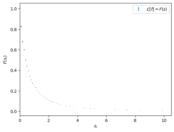
To demonstrate this, we first generate mock data corresponding to \(F(s)\) and will then try to find (our secretly known) \(f(t)\).

epsilon = 0.01  # 1 percent noise
s_data = np.linspace(0, 10, 101)
F_data = laplace_model(s=s_data).F
F_sigma = epsilon * F_data
np.random.seed(2)
F_data = np.random.normal(F_data, F_sigma)

plt.errorbar(s_data, F_data, yerr=F_sigma, fmt='none', label=r'$\mathcal{L}[f] = F(s)$')
plt.xlabel(r'$s_i$')
plt.ylabel(r'$F(s_i)$')
plt.xlim(0, None)
plt.legend()

<matplotlib.legend.Legend at 0x7f4c32531e10>

We will now invert this data, using the procedure outlined in \cite{}.

N_s = symbols('N_s', integer=True)  # Number of s_i points

M = MatrixSymbol('M', N_s, N_s)
W = MatrixSymbol('W', N_s, N_s)
Fs = MatrixSymbol('Fs', N_s, 1)
c = MatrixSymbol('c', N_s, 1)
d = MatrixSymbol('d', 1, 1)
I = MatrixSymbol('I', N_s, N_s)
a, = parameters('a')

model_dict = {
    W: Inverse(I + M / a**2),
    c: - W * Fs,
    d: sqrt(c.T * c),
}
tikhonov_model = CallableModel(model_dict)
print(tikhonov_model)

[W(I, M; a) = (I + a**(-2)*M)**(-1),
 c(Fs, W; ) = -W*Fs,
 d(c; ) = (c.T*c)**(1/2)]

A CallableModel is needed because derivatives of matrix expressions sometimes cause problems.

Build required matrices, ignore s=0 because it causes a singularity.

I_mat = np.eye(len(s_data[1:]))
s_i, s_j = np.meshgrid(s_data[1:], s_data[1:])
M_mat = 1 / (s_i + s_j)
delta = np.atleast_2d(np.linalg.norm(F_sigma))
print('d', delta)

d [[0.01965714]]

Perform the fit

model_data = {
    I.name: I_mat,
    M.name: M_mat,
    Fs.name: F_data[1:],
}
all_data = dict(**model_data, **{d.name: delta})

fit = Fit(tikhonov_model, **all_data)
fit_result = fit.execute()
print(fit_result)

Parameter Value        Standard Deviation
a         5.449374e-02 None
Status message         Optimization terminated successfully.
Number of iterations   14
Objective              <symfit.core.objectives.LeastSquares object at 0x7f4c30478790>
Minimizer              <symfit.core.minimizers.BFGS object at 0x7f4c3313ed50>

Goodness of fit qualifiers:
chi_squared            3.289863264548032e-19
objective_value        1.644931632274016e-19
r_squared              -inf

/home/docs/checkouts/readthedocs.org/user_builds/symfit/envs/stable/lib/python3.7/site-packages/symfit/core/fit_results.py:279: RuntimeWarning: divide by zero encountered in double_scalars
  return 1 - SS_res/SS_tot

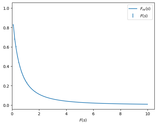
Check the quality of the reconstruction

ans = tikhonov_model(**model_data, **fit_result.params)
F_re = - M_mat.dot(ans.c) / fit_result.value(a)**2
print(ans.c.shape, F_re.shape)

plt.errorbar(s_data, F_data, yerr=F_sigma, label=r'$F(s)$', fmt='none')
plt.plot(s_data[1:], F_re, label=r'$F_{re}(s)$')
plt.xlabel(r'$x$')
plt.xlabel(r'$F(s)$')
plt.xlim(0, None)
plt.legend()

(100,) (100,)

<matplotlib.legend.Legend at 0x7f4c302a7190>

Reconstruct \(f(t)\) and compare with the known original.

t_data = np.linspace(0, 10, 101)
f_data = model(t=t_data).f
f_re_func = lambda x: - np.exp(- x * s_data[1:]).dot(ans.c) / fit_result.value(a)**2
f_re = [f_re_func(t_i) for t_i in t_data]

plt.axhline(0, color='black')
plt.axvline(0, color='black')
plt.plot(t_data, f_data, label=r'$f(t)$')
plt.plot(t_data, f_re, label=r'$f_{re}(t)$')
plt.xlabel(r'$t$')
plt.xlabel(r'$f(t)$')
plt.legend()

<matplotlib.legend.Legend at 0x7f4c3015ca10>

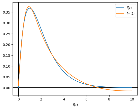
Not bad, for an ill-defined problem.