Example: Piecewise continuous function
Piecewise continuus functions can be tricky to fit. However, using the
symfit interface this process is made a lot easier. Suppose we want to
fit to the following model:
\[\begin{split}f(x) = \begin{cases} x^2 - a x & \text{if}\quad x \leq x_0 \\
a x + b & \text{otherwise}
\end{cases}\end{split}\]
The script below gives an example of how to fit such a model:
from symfit import parameters, variables, Fit, Piecewise, exp, Eq, Model
import numpy as np
import matplotlib.pyplot as plt

x, y = variables('x, y')
a, b, x0 = parameters('a, b, x0')

# Make a piecewise model
y1 = x**2 - a * x
y2 = a * x + b
model = Model({y: Piecewise((y1, x <= x0), (y2, x > x0))})

# As a constraint, we demand equality between the two models at the point x0
# to do this, we substitute x -> x0 and demand equality using `Eq`
constraints = [
    Eq(y1.subs({x: x0}), y2.subs({x: x0}))
]
# Generate example data
xdata = np.linspace(-4, 4., 50)
ydata = model(x=xdata, a=0.0, b=1.0, x0=1.0).y
np.random.seed(2)
ydata = np.random.normal(ydata, 0.5)  # add noise

# Help the fit by bounding the switchpoint between the models
x0.min = 0.8
x0.max = 1.2

fit = Fit(model, x=xdata, y=ydata, constraints=constraints)
fit_result = fit.execute()
print(fit_result)

plt.scatter(xdata, ydata)
plt.plot(xdata, model(x=xdata, **fit_result.params).y)
plt.show()
This code prints:
Parameter Value        Standard Deviation
a         -4.780338e-02 None
b         1.205443e+00 None
x0        1.051163e+00 None
Fitting status message: Optimization terminated successfully.
Number of iterations:   18
Regression Coefficient: 0.9849188499599985
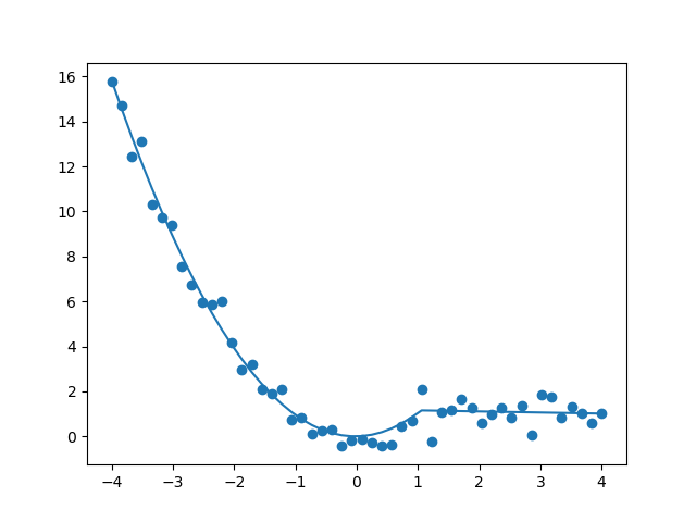
Judging from this graph, another possible solution would have been to also demand a continuous derivative at the point x0. This can be achieved by setting the following constraints instead:
constraints = [
    Eq(y1.diff(x).subs({x: x0}), y2.diff(x).subs({x: x0})),
    Eq(y1.subs({x: x0}), y2.subs({x: x0}))
]
This gives the following plot:
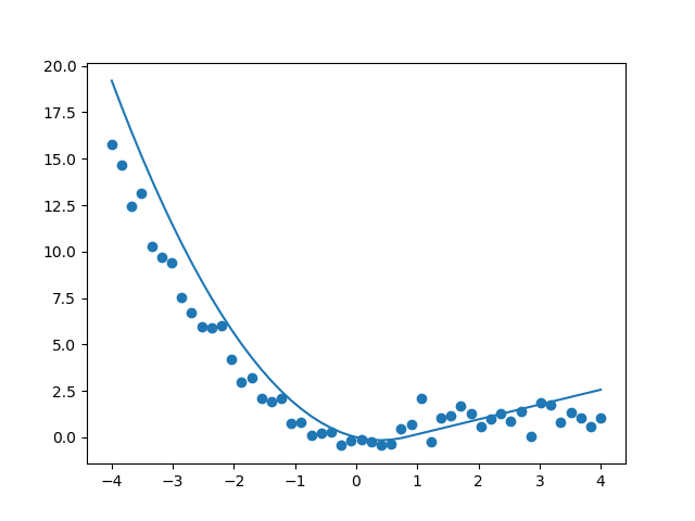
and the following fit report:
Parameter Value        Standard Deviation
a         8.000000e-01 None
b         -6.400000e-01 None
x0        8.000000e-01 None
Fitting status message: Optimization terminated successfully.
Number of iterations:   3
Regression Coefficient: 0.8558226069368662
The first fit is therefore the prevered one, but it does show you how easy it is
to set these constraints using symfit.