Example: ODEModel for Reaction Kinetics
Below is an example of how to use the symfit.core.models.ODEModel. In
this example we will fit reaction kinetics data, taken from libretexts.
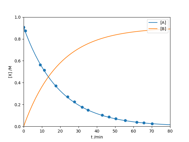
The data is from a first-order reaction \(\text{A} \rightarrow \text{B}\).
from symfit import variables, Parameter, Fit, D, ODEModel
import numpy as np
import matplotlib.pyplot as plt

# First order reaction kinetics. Data taken from
# http://chem.libretexts.org/Core/Physical_Chemistry/Kinetics/Rate_Laws/The_Rate_Law
tdata = np.array([0, 0.9184, 9.0875, 11.2485, 17.5255, 23.9993, 27.7949,
                  31.9783, 35.2118, 42.973, 46.6555, 50.3922, 55.4747, 61.827,
                  65.6603, 70.0939])
concentration = np.array([0.906, 0.8739, 0.5622, 0.5156, 0.3718, 0.2702, 0.2238,
                          0.1761, 0.1495, 0.1029, 0.086, 0.0697, 0.0546, 0.0393,
                          0.0324, 0.026])

# Define our ODE model
A, B, t = variables('A, B, t')
k = Parameter('k')
model = ODEModel(
    {D(A, t): - k * A, D(B, t): k * A},
    initial={t: tdata[0], A: concentration[0], B: 0.0}
)

fit = Fit(model, A=concentration, t=tdata)
fit_result = fit.execute()

print(fit_result)

# Plotting, irrelevant to the symfit part.
t_axis = np.linspace(0, 80)
A_fit, B_fit, = model(t=t_axis, **fit_result.params)
plt.scatter(tdata, concentration)
plt.plot(t_axis, A_fit, label='[A]')
plt.plot(t_axis, B_fit, label='[B]')
plt.xlabel('t /min')
plt.ylabel('[X] /M')
plt.ylim(0, 1)
plt.xlim(0, 80)
plt.legend(loc=1)
plt.show()
This is the resulting fit: